Code
library(tidyverse)
library(ggplot2)
library(tidymodels)
library(rsample)
library(themis)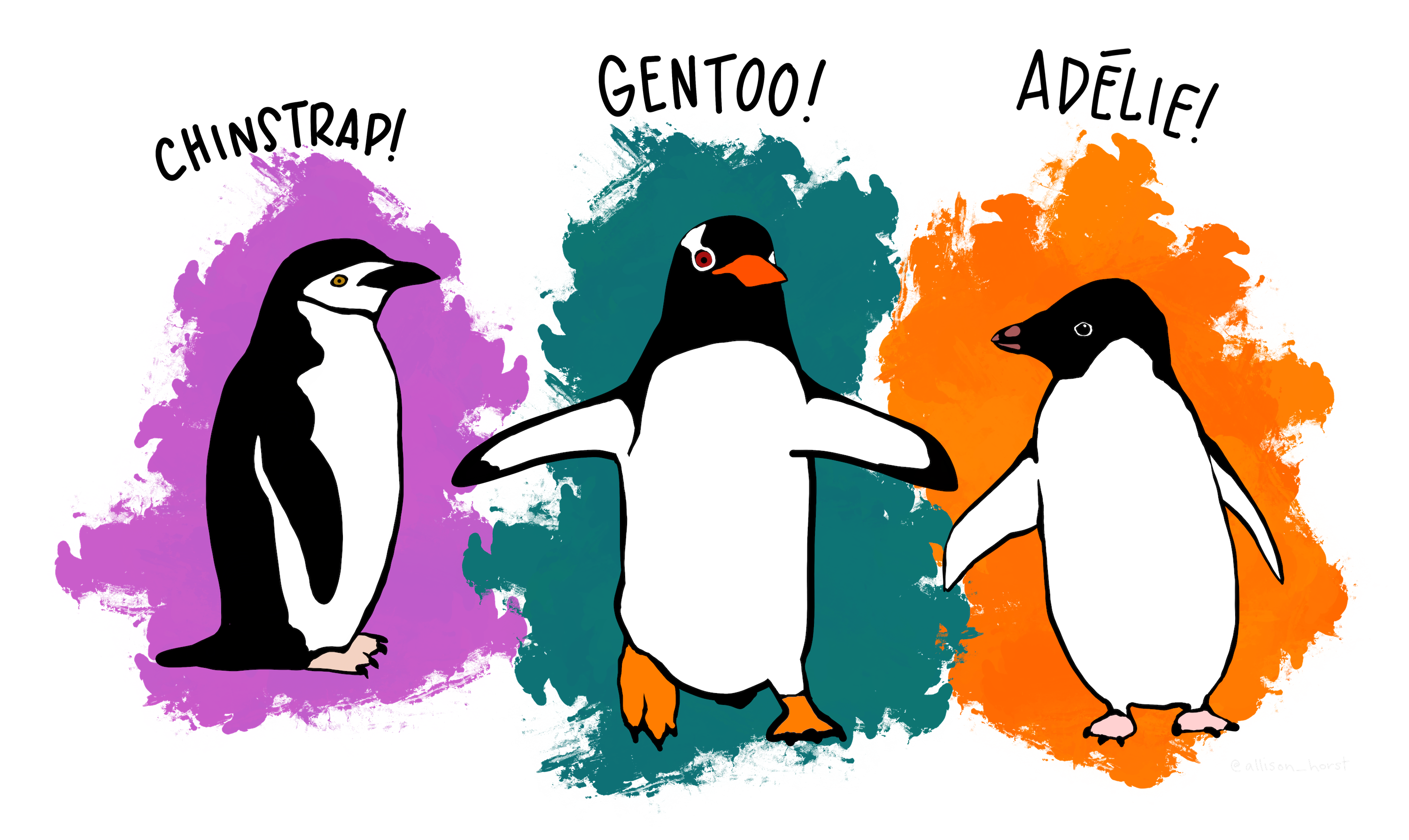
library(tidyverse)
library(ggplot2)
library(tidymodels)
library(rsample)
library(themis)library(tidyverse)
library(palmerpenguins)
head(penguins)# A tibble: 6 × 8
species island bill_length_mm bill_depth_mm flipper_length_mm body_mass_g
<fct> <fct> <dbl> <dbl> <int> <int>
1 Adelie Torgersen 39.1 18.7 181 3750
2 Adelie Torgersen 39.5 17.4 186 3800
3 Adelie Torgersen 40.3 18 195 3250
4 Adelie Torgersen NA NA NA NA
5 Adelie Torgersen 36.7 19.3 193 3450
6 Adelie Torgersen 39.3 20.6 190 3650
# ℹ 2 more variables: sex <fct>, year <int>glimpse(penguins)Rows: 344
Columns: 8
$ species <fct> Adelie, Adelie, Adelie, Adelie, Adelie, Adelie, Adel…
$ island <fct> Torgersen, Torgersen, Torgersen, Torgersen, Torgerse…
$ bill_length_mm <dbl> 39.1, 39.5, 40.3, NA, 36.7, 39.3, 38.9, 39.2, 34.1, …
$ bill_depth_mm <dbl> 18.7, 17.4, 18.0, NA, 19.3, 20.6, 17.8, 19.6, 18.1, …
$ flipper_length_mm <int> 181, 186, 195, NA, 193, 190, 181, 195, 193, 190, 186…
$ body_mass_g <int> 3750, 3800, 3250, NA, 3450, 3650, 3625, 4675, 3475, …
$ sex <fct> male, female, female, NA, female, male, female, male…
$ year <int> 2007, 2007, 2007, 2007, 2007, 2007, 2007, 2007, 2007…penguins %>%
count(species)# A tibble: 3 × 2
species n
<fct> <int>
1 Adelie 152
2 Chinstrap 68
3 Gentoo 124library(skimr)
skim(penguins)| Name | penguins |
| Number of rows | 344 |
| Number of columns | 8 |
| _______________________ | |
| Column type frequency: | |
| factor | 3 |
| numeric | 5 |
| ________________________ | |
| Group variables | None |
Variable type: factor
| skim_variable | n_missing | complete_rate | ordered | n_unique | top_counts |
|---|---|---|---|---|---|
| species | 0 | 1.00 | FALSE | 3 | Ade: 152, Gen: 124, Chi: 68 |
| island | 0 | 1.00 | FALSE | 3 | Bis: 168, Dre: 124, Tor: 52 |
| sex | 11 | 0.97 | FALSE | 2 | mal: 168, fem: 165 |
Variable type: numeric
| skim_variable | n_missing | complete_rate | mean | sd | p0 | p25 | p50 | p75 | p100 | hist |
|---|---|---|---|---|---|---|---|---|---|---|
| bill_length_mm | 2 | 0.99 | 43.92 | 5.46 | 32.1 | 39.23 | 44.45 | 48.5 | 59.6 | ▃▇▇▆▁ |
| bill_depth_mm | 2 | 0.99 | 17.15 | 1.97 | 13.1 | 15.60 | 17.30 | 18.7 | 21.5 | ▅▅▇▇▂ |
| flipper_length_mm | 2 | 0.99 | 200.92 | 14.06 | 172.0 | 190.00 | 197.00 | 213.0 | 231.0 | ▂▇▃▅▂ |
| body_mass_g | 2 | 0.99 | 4201.75 | 801.95 | 2700.0 | 3550.00 | 4050.00 | 4750.0 | 6300.0 | ▃▇▆▃▂ |
| year | 0 | 1.00 | 2008.03 | 0.82 | 2007.0 | 2007.00 | 2008.00 | 2009.0 | 2009.0 | ▇▁▇▁▇ |
penguins %>%
  filter(!is.na(sex)) %>%
  ggplot(aes(flipper_length_mm, bill_length_mm, color = sex, size = body_mass_g)) +
  geom_point(alpha = 0.5) +
  facet_wrap(~species)
penguins_df <- penguins %>%
  filter(!is.na(sex)) %>%
select(-year, -island)library(tidymodels)
set.seed(123)
penguin_split <- initial_split(penguins_df, strata = sex)
penguin_train <- training(penguin_split)
penguin_test <- testing(penguin_split)set.seed(123)
penguin_boot <- bootstraps(penguin_train)
penguin_boot# Bootstrap sampling
# A tibble: 25 × 2
splits id
<list> <chr>
1 <split [249/93]> Bootstrap01
2 <split [249/91]> Bootstrap02
3 <split [249/90]> Bootstrap03
4 <split [249/91]> Bootstrap04
5 <split [249/85]> Bootstrap05
6 <split [249/87]> Bootstrap06
7 <split [249/94]> Bootstrap07
8 <split [249/88]> Bootstrap08
9 <split [249/95]> Bootstrap09
10 <split [249/89]> Bootstrap10
# ℹ 15 more rowsdid not use recipe at this case
glm_spec <- logistic_reg() %>%
set_engine("glm")glm_specLogistic Regression Model Specification (classification)
Computational engine: glm rf_spec <- rand_forest() %>%
set_mode("classification") %>%
set_engine("ranger")rf_specRandom Forest Model Specification (classification)
Computational engine: ranger penguin_wf <- workflow() %>%
add_formula(sex ~ .)penguin_wf══ Workflow ════════════════════════════════════════════════════════════════════
Preprocessor: Formula
Model: None
── Preprocessor ────────────────────────────────────────────────────────────────
sex ~ .glm_rs <- penguin_wf %>%
add_model(glm_spec) %>%
fit_resamples(
resamples = penguin_boot,
control = control_resamples(save_pred = TRUE)
)glm_rs# Resampling results
# Bootstrap sampling
# A tibble: 25 × 5
splits id .metrics .notes .predictions
<list> <chr> <list> <list> <list>
1 <split [249/93]> Bootstrap01 <tibble [2 × 4]> <tibble [0 × 3]> <tibble>
2 <split [249/91]> Bootstrap02 <tibble [2 × 4]> <tibble [0 × 3]> <tibble>
3 <split [249/90]> Bootstrap03 <tibble [2 × 4]> <tibble [0 × 3]> <tibble>
4 <split [249/91]> Bootstrap04 <tibble [2 × 4]> <tibble [0 × 3]> <tibble>
5 <split [249/85]> Bootstrap05 <tibble [2 × 4]> <tibble [1 × 3]> <tibble>
6 <split [249/87]> Bootstrap06 <tibble [2 × 4]> <tibble [0 × 3]> <tibble>
7 <split [249/94]> Bootstrap07 <tibble [2 × 4]> <tibble [0 × 3]> <tibble>
8 <split [249/88]> Bootstrap08 <tibble [2 × 4]> <tibble [1 × 3]> <tibble>
9 <split [249/95]> Bootstrap09 <tibble [2 × 4]> <tibble [0 × 3]> <tibble>
10 <split [249/89]> Bootstrap10 <tibble [2 × 4]> <tibble [0 × 3]> <tibble>
# ℹ 15 more rows
There were issues with some computations:
- Warning(s) x3: glm.fit: fitted probabilities numerically 0 or 1 occurred
Run `show_notes(.Last.tune.result)` for more information.rf_rs <- penguin_wf %>%
add_model(rf_spec) %>%
fit_resamples(
resamples = penguin_boot,
control = control_resamples(save_pred = TRUE)
)rf_rs# Resampling results
# Bootstrap sampling
# A tibble: 25 × 5
splits id .metrics .notes .predictions
<list> <chr> <list> <list> <list>
1 <split [249/93]> Bootstrap01 <tibble [2 × 4]> <tibble [0 × 3]> <tibble>
2 <split [249/91]> Bootstrap02 <tibble [2 × 4]> <tibble [0 × 3]> <tibble>
3 <split [249/90]> Bootstrap03 <tibble [2 × 4]> <tibble [0 × 3]> <tibble>
4 <split [249/91]> Bootstrap04 <tibble [2 × 4]> <tibble [0 × 3]> <tibble>
5 <split [249/85]> Bootstrap05 <tibble [2 × 4]> <tibble [0 × 3]> <tibble>
6 <split [249/87]> Bootstrap06 <tibble [2 × 4]> <tibble [0 × 3]> <tibble>
7 <split [249/94]> Bootstrap07 <tibble [2 × 4]> <tibble [0 × 3]> <tibble>
8 <split [249/88]> Bootstrap08 <tibble [2 × 4]> <tibble [0 × 3]> <tibble>
9 <split [249/95]> Bootstrap09 <tibble [2 × 4]> <tibble [0 × 3]> <tibble>
10 <split [249/89]> Bootstrap10 <tibble [2 × 4]> <tibble [0 × 3]> <tibble>
# ℹ 15 more rowscollect_metrics(rf_rs)# A tibble: 2 × 6
.metric .estimator mean n std_err .config
<chr> <chr> <dbl> <int> <dbl> <chr>
1 accuracy binary 0.914 25 0.00545 Preprocessor1_Model1
2 roc_auc binary 0.977 25 0.00202 Preprocessor1_Model1collect_metrics(glm_rs)# A tibble: 2 × 6
.metric .estimator mean n std_err .config
<chr> <chr> <dbl> <int> <dbl> <chr>
1 accuracy binary 0.918 25 0.00639 Preprocessor1_Model1
2 roc_auc binary 0.979 25 0.00254 Preprocessor1_Model1glm_rs %>%
conf_mat_resampled()# A tibble: 4 × 3
Prediction Truth Freq
<fct> <fct> <dbl>
1 female female 41.1
2 female male 3
3 male female 4.4
4 male male 42.3penguin_final <- penguin_wf %>%
add_model(glm_spec) %>%
last_fit(penguin_split)
penguin_final# Resampling results
# Manual resampling
# A tibble: 1 × 6
splits id .metrics .notes .predictions .workflow
<list> <chr> <list> <list> <list> <list>
1 <split [249/84]> train/test split <tibble> <tibble> <tibble> <workflow>collect_metrics(penguin_final)# A tibble: 2 × 4
.metric .estimator .estimate .config
<chr> <chr> <dbl> <chr>
1 accuracy binary 0.857 Preprocessor1_Model1
2 roc_auc binary 0.938 Preprocessor1_Model1collect_predictions(penguin_final) %>%
conf_mat(sex, .pred_class) Truth
Prediction female male
female 37 7
male 5 35penguin_final$.workflow[[1]] %>%
tidy(exponentiate = TRUE)# A tibble: 7 × 5
term estimate std.error statistic p.value
<chr> <dbl> <dbl> <dbl> <dbl>
1 (Intercept) 5.75e-46 19.6 -5.31 0.000000110
2 speciesChinstrap 1.37e- 4 2.34 -3.79 0.000148
3 speciesGentoo 1.14e- 5 3.75 -3.03 0.00243
4 bill_length_mm 1.91e+ 0 0.180 3.60 0.000321
5 bill_depth_mm 8.36e+ 0 0.478 4.45 0.00000868
6 flipper_length_mm 1.06e+ 0 0.0611 0.926 0.355
7 body_mass_g 1.01e+ 0 0.00176 4.59 0.00000442 https://www.youtube.com/watch?v=z57i2GVcdww
https://juliasilge.com/blog/palmer-penguins/